Trigonometric functions are basically the function of an angle in relation with a right triangle. For the purpose of our Processing study we are going to describe the trigonometric functions in terms of their drawing capabilities, the reason for taken this approach to explain these functions is that it will make our understanding of Processing programming much easier. The trigonometric functions are:
• Sine
• Cosine
• Tangent
The Sine function
To help us visualize these functions it is useful to define them with the help of the ‘unit circle’. A unit circle is a circle, which has a radius (r), of 1 unit in length.
Let’s think, for example, of the following picture as being a wheel, with centre C= 0, 0. The point P is the intersection of the line, with length r, traced from the centre to the edge (the circumference) of the wheel. Also note that the point P is following the circumference of the wheel in an anti-clockwise movement.


Now, let’s trace a perpendicular line from point P ending on the horizontal axis, X, and we do this for every point P on the circumference, as in figure 1.2

We can easily see that for every point on the circumference we end up with an infinite number of perpendicular lines (in blue) on the X-axis, Y. It is this line that we are interested in, as it corresponds to the function sine of the angle theta, sin (θ).
For the mathematical minded and for those that need to come to terms why this is so, please refer to box ‘Note B’. It defines the trigonometric functions of an angle (θ) in relation to a righted-triangle; that is, as ratios of the lengths of the triangle sides.

OK, we now are going to see how sin (θ) provides us with the power to graphics programming.
We now draw the movement of the point P in a x-y coordinates plane (the Cartesian plane), with horizontal axis X and vertical axis Y, as it circles around the wheel.
We need to plot on the axis Y the positive and negative value of 1 unit and on axis X the value of the angle theta that P has travel along the wheel, against time, in this example 1 second.
The result is illustrated in the following graph:

Clearly, figure 2 shows the graphic characteristics of a sine function, a sine wave. Here point P has travel 360 degrees (or 2π radians); in other words one revolution.
If P were to carry on rotating along the circumference of the wheel more than 1 revolution, then we will have a periodic sine function. This means that in the graph the wiggly line will continue towards infinity.
The amplitude, that is, the magnitude of the radius of the wheel on our example can have any other value, making the wheel smaller or bigger.
The Cosine function
As with the sine function the cosine function can be demonstrated to possess graphics properties. This time, however, we are concerned with the adjacent side of the angle theta, X (in red).

Remember from the facts listed in 'Note B' above, we can conclude that because:
cos(θ) = adjacent/hypotenuse
cos(θ) = X/1 = X (expression 2)
Therefore, when theta, θ, is:
0° then cos(θ) = X = 1, the radius.
90° then cos(θ) = X = 0
180° then cos(θ) = X = -1
270° then cos(θ) = X = 0
360° then cos(θ) = X = 1
The following figure illustrates the cosine function graphed on the Cartesian plane, in which we can note another kind of wave:

Again, point P has travelled a complete revolution and if it were to carry on it will result on a periodic cosine wave.
Comparison between Sine and Cosine functions
We are now going to compare these two functions. To do that we can overlap the two graphs, imagining one on top of the other, like this:

Figure 5 we can observe a relationship between the two functions. The sine wave can be considered identical to a cosine wave, but they are separated by one quarter of a cycle; that is π/2 radians. In other words, the cosine leads the sine wave by 90 degrees.
As we seen in 'Note B', the sine and cosine functions are translated into the Cartesian plane by:
X = cos(θ) * radius (expression 3)
Y = sin(θ) * radius (expression 4)
Note that these expressions are deducted from expression2 and expression 1 respectively.
This is how we can plot the point P into the Cartesian plane with axis y and x. Now, we are interested in translating these expressions for use in our Processing programming.
The following are the trigonometric functions in Processing:
float x = cos(radians(angle)) * radius (expression 5)
float y = sin(radians(angle)) * radius (expression 6)
Please note the difference between using degrees and radians for measuring the angle theta. Here the function radians(angle) is used to give the angle in radians.
Demonstration of the Sine function in relation with the unit circle
The following is a simple program, 'SineWave', to demonstrate the relationship between the unit circle and the Sine function:
// initialising variables
float Y = 0;
float X = 0;
float Cx = 90;
float Cy =150;
float radius = 75;
float theta = 0;
int i = 188;
PFont font;
String label = "π/2 π 3π/2 2π";
boolean last = false;
// set up frame, circle and coordinates plane
void setup() {
size (590, 350);
fill(255);
strokeWeight(1);
ellipse(Cx, Cy, 150, 150);
// draw cartesian plane
strokeWeight(1);
line(Cx, Cy, Cx+480, 150);
line(191, 65, 191, 250);
// write labels
fill(0);
font = createFont("Helvetica", 32);
textFont(font, 13);
text(label, 270, 168);
}
//draw the sine function in the cartesian plane
void draw()
{
if (theta <= 360)
{
// when the last horizontal line has been drawn
// then change to white colour, so that leading line is black
if (last)
{
stroke(199);
strokeWeight(1);
line(Cx + X, Cy - Y, i, Cy - Y);
if(theta == 185)
{
stroke(0);
line(191, Cy - Y, i, Cy - Y);
}
}
// axis x and y
strokeWeight(1);
Y = sin(radians(theta))* radius;
X = cos(radians(theta))* radius;
// slow down
try {
Thread.sleep(270);
}
catch (Exception e) {}
// draw the radius
stroke(0); // black radius
line(Cx, Cy, Cx + X, Cy - Y);
// draw the blue point in circunference
strokeWeight(5); // thick dot
stroke(20, 180, 250); // blue
point(Cx + X, Cy - Y);
// draw sine wave in axis coordinates, a series of blue dots
i = i + 5;
point (i, Cy - Y);
// draw a line to joint blue point with sine wave
stroke(0);
strokeWeight(1);
line(Cx + X, Cy - Y, i, Cy - Y);
theta = theta + 5; // increment angle
}
last = true; // last line drew
}

Some Examples
Now that we know the way to graph sine and cosine functions using Processing, we can start with a very simple program. Let’s call it ‘Coloured_ waves’, which just draw two sine waves differing in colour, see figure 7.
// initialising variables
int y = 100; // the screen vertical coordinate
float S = 0; // sine value/y coordinate float
theta = 0; // angle
float amplitude = 60; // radius
// set up window
size (400, 300);
strokeWeight(3);// thickness of point
// draw the first wave of green colour
stroke(0, 190, 0); // green
for (int i = 10; i <= 380; i=i + 2)
{
S = sin(radians(theta))*amplitude;
point (i, y - S);
theta = theta + 3;
}
// draw a second wave of orange colour
stroke(255, 128, 0); // orange
theta =0;
y = 200;
for (int i = 10; i <= 380; i=i + 2)
{
S = sin(radians(theta))*amplitude;
point (i, y - S);
theta = theta + 3;
}

So now we could become a little more adventurous in our programming.
The next program is called ‘Alternated_Waves’ and it draws a series of cosines waves with its directions alternated. The waves in black colour can be seen as mirrored by the waves in purple. Figure 8 shows the result.
// var initialising
int y = 75;
float theta = 0;
void setup() {
size(500, 500);
background(255);
strokeWeight(3);
}
void draw(){
float cosine = 0;
if (y < 425)
{
// j represents times cosine function will draw in screen
for (int j = 1; j <= 6; j++)
{
theta = 0;
// i is the lenght of the cosine wave across the screen
for (int i = 20; i < 453; i++)
{
if ((j+1)%2 == 0)
{
stroke(0);
cosine = cos(radians(theta))*(35);
point(i, cosine + y);
theta = theta + 5;
}
else
{
stroke(180, 35, 255); // purple
cosine = cos(radians(theta))*(35);
point(i, y - cosine);
theta = theta + 5;
}
}
y = y + 70;
}
}
}

The tangent function
Once sine and cosine functions have been defined we can derive the tangent function from these two.
Recalling from ‘Note B’, we have the expression:
tan(θ) = Opposite/Adjacent
Now lets repeat our figure of the unit circle but this time showing both sine and cosine functions, like this:

In figure 9 we can see the line, highlighted in green (Z), which corresponds to the tangent function forming a perpendicular with the radius on point P. We could say that the tangent just touches the unit circle at point P.
Therefore we have:
tan(θ) = Opposite/Adjacent = Y/X
Also recall expressions 1 and 2, repeated here:
sin(θ) = Y/1 = Y (expression 1)
cos(θ) = X/1 = X (expression 2)
Therefore we can conclude that:
tan(θ) = sin(θ) / cos(θ)
Lets calculate values of tangent when theta , θ, equals:
0° then tan(θ) = Y/X = 0/1 = 0
90° then tan(θ) = Y/X = 1/0 = undefined
180° then tan(θ) = Y/X = 0/-1 = 0
270° then tan(θ) = Y/X = -1/0 = undefined
360° then tan(θ) = Y/X = 0/1 = 0
Finally, the Processing expression to program the tangent function is:
float z = tan(radians(angle)) * radius (expression 7)
The following program, ‘TangentWave’, draws the tangent for one revolution on the Cartesian plane.
// initialising variables
float tang = 0;
float Y = 0;
float X = 0;
float Cx = 100;
float Cy = 350;
float radius = 75;
float theta = 0;
int i = 188;
PFont font;
String label = "π/2 π 3π/2 2π";
boolean last = false;
// set up frame, circle and coordinates plane
void setup() {
size (600, 700);
fill(255);
strokeWeight(1);
ellipse(Cx, Cy, 150, 150);
// draw cartesian plane
strokeWeight(1);
line(Cx, Cy, Cx+465, Cy);
line(191, 250, 191, 500);
stroke(185);
line(270, 50, 270, 660);
line(450, 50, 450, 660);
// write labels
fill(0);
font = createFont("Helvetica", 32);
textFont(font, 15);
text(label, 271, 370);
}
//draw the tangent function in the cartesian plane
void draw()
{
if (theta <= 360)
{
// when the last horizontal line has been drawn
// then change to grey, so that leading line is black
if (last)
{
stroke(185); // grey
strokeWeight(1);
line(Cx + X, Cy - tang, i, Cy - tang);
if(theta == 185)
{
stroke(0);
line(191, Cy - tang, i, Cy - tang);
}
}
// axis x and y
strokeWeight(1);
tang = tan(radians(theta))*radius;
Y = sin(radians(theta))*radius;
X = cos(radians(theta))*radius;
// slow down
try {
Thread.sleep(270);
}
catch (Exception e) {}
// draw the angle line, radius
stroke(185); // grey radius
line(Cx, Cy, Cx + X, Cy - Y);
// draw the point that follows the tangent
strokeWeight(3); // dot thickness
stroke(20, 180, 250); // blue
point(Cx + X, Cy - tang);
// draw sine wave in axis coordinates, a series of green dots
strokeWeight(6); // thick dot
stroke(30, 200, 175); // green
i = i + 5;
point (i, Cy - tang);
// draw a line to joint tangent point with tangent wave
stroke(0);
strokeWeight(1);
line(Cx + X, Cy - tang, i, Cy - tang);
theta = theta + 5; // increment angle
}
last = true; // last line drew
}
The result is shown in figure 10 below.
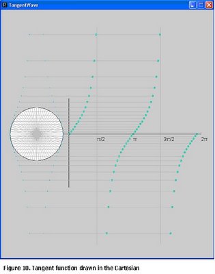
The figure above illustrate a different curve altogether from those of the sine and cosine functions. We can see that at 90 and 270 degrees (π/2 and 3π/2 radians respectively) the curve is undefined, going upwards towards positive infinity (+ Y) at 90 degrees and reappearing on the negative coordinate Y at 91 degrees. The same can be said when theta is at 270, 450, etc.
Again, if we can carry on further than one revolution, we will be able to see that there is a repeating pattern at every 180 degrees. For example, in figure 10 we can see a curve formed between angles 90 (π/2) and 270 (3π/2) degrees, this shape of curve will repeat at angles between 270 and 450, and between 450 and 630 degreees and so on.
--- Let’s make art ---
OK, we have now defined and understood where these three fundamental trigonometric functions come from and as you might agree this is a very interesting and easy way to help our understanding and we hope this have opened your appetite for further investigation and experimentation.
The program that follows draws a flower designed with the trigonometric functions. It has been named ‘Trigo_Flower’ and the result is illustrated in figure 11.
The flower is drawn from the centre of the window. At its centre there is a small bright purple circle. The flower has a distinctive centre also in blue. The ‘petals’ are drawn in dark purple, with the outer petal drawn a 2/3 of its way in light purple. The gap between second and third petal has been filled with light purple, giving an elegant finish to the flower. These have been achieved with the sine function.
And finally, the tangent function is used as a way to simulate the filaments containing the pollen, in dark purple. Also, tangent is used to draw the leaves on each corner of the window.
Here is the code for the ‘Trigo_Flower’ program.
// var initialising
float Y = 0; // sine function
float X = 0; // cosine function
float tang = 0; // tangent function
// for x and y coordinates
float Cx = 0; // x coordinate
float Cy =0; // y coordinate
float Cx1 = 0;
float Cx2 = 0;
// angles
float theta = 0;
float betha = 0;
float centre = 250; // the centre of window
// set up window
void setup() {
size(500, 500);
background(255);
strokeWeight(3);
}
// draw flower function
void draw(){
float temp1 = 0;
float y = 0; // sine
if (betha <= 360)
{
// calculate trig functions. Radius is 183, the flower will fit in this circle
Y = sin(radians(betha))* 183;
X = cos(radians(betha))* 183;
// calculate the coordinates, it is centred in the centre of window
Cx = width/2 + X;
Cy = height/2 - Y;
// when angle is 45 degrees calculate coordinates
// to shorten petal
if (betha == 45)
{
Cx1 = width/2 + X; // coor x to the right
Cx2 = width/2 - X; // coor x to the left
}
/* ---------drawing the flower------------*/
theta = 0;
if (theta <= 360)
{
strokeWeight(5); // thick dot
stroke(20, 180, 250); // blue
// draw and paint centre of flower, blue
for (float i = 160; i <= 335; i++)
{
y = sin(radians(theta))*20/4;
point(y + centre, i); // sine function drawn from bottom to top/rigth to left
point(centre - y, i); // sine function drawn from top to bottom/left to right
point(i, centre - y); // sine function drawn from rigth to left/bottom to top
point(i , y + centre ); // sine function drawn from left to right/top to bottom
theta++;
}
// to fill the centre
theta = 0;
for (float i = 175; i <= 320; i++)
{
y = sin(radians(theta))*20/13;
point(y + centre, i);
point(centre - y, i);
point(i, centre - y);
point(i , y + centre );
theta++;
}
// carry on drawing, draw first petal with radius 20
theta =0;
strokeWeight(3);
for (int i = 75; i <= Cy; i++)
{
stroke(115, 10, 255); // dark purple
y = sin(radians(theta))*20;
point(y + centre, i);
point(centre - y, i);
point(i, centre - y);
point(i, y + centre);
// colour gap between outer and inner petals
stroke(190, 90, 245); // back to purple
temp1 = 38; // starting radius
for (int j=1; j <= 17; j= j+1)
{
y = sin(radians(theta))*temp1;
point(y + centre, i);
point(centre - y, i);
point(i, y + centre);
point(i, centre - y);
temp1= temp1 - 1; // decreasing radius
}
theta++;
}
// ---------- draw bigger petal, radius 40 --------------
theta = 0;
for (int i = 75; i <= Cx; i++)
{
stroke(115, 10, 255); // dark purple
y = sin(radians(theta))*40;
point(y + centre, i);
point(i, centre - y);
point(i, y + centre );
point(centre - y, i);
// draw purple tangent function across flower for decoration as pollen filaments
if ((theta > 100) && (theta < 260))
{
stroke(115, 10, 255); // dark purple
tang = tan(radians(theta ))*30;
point(i, tang + centre);
point(centre - tang, i);
point(tang + centre, i);
point(i, centre - tang);
}
theta++;
}
// ------------- draw last petal leaving a one third of it empty -----------------
theta = 0;
for (float i = 75 ; i <= Cx1; i++)
{
stroke(190, 90, 245); // back to purple
if (i >= Cx2)
{
y = sin(radians(theta))*55;
point(y + centre, i);
point(i, centre - y);
point(i , y + centre );
point(centre - y, i);
}
theta++;
}
// --------------- draw green leaves ----------------
theta = 165;
for (int i = 25; i <= 155; i=i+1)
{
if ((theta > 165) && (theta < 260))
{
stroke(10, 140, 65); // green
for (int k = 25; k <= 35; k= k + 1)
{
tang = tan(radians(theta))*10;
// top-left leaf
point(i, tang + k);
point(tang + k, i );
// top-right leaf
point(width - i, tang + k);
point(width-(tang+k),i );
// bottom-left
point(tang + k, width - i);
point(i, width - (tang+k));
// bottom-right
point(width - i, width-(tang + k));
point(width - (tang+k), width - i);
}
}
theta++;
}
// inside each leaf
theta = 160;
temp1 = 15.5;
for (int i = 25; i <= 130; i=i+2)
{
if ((theta > 175) && (theta < 230))
{
tang = tan(radians(theta))*(temp1);
temp1 = temp1 + 2.5;
// top-left corner
point(i, tang + 65);
point(tang + 65, i);
// top-right corner
point(width -i, tang+65);
point(width-(tang+65),i );
// bottom-left
point(tang+65, width-i);
point(i, width - (tang+65));
// bottom-right
point(width - i, width-(tang + 65));
point(width - (tang+65), width - i);
}
theta++;
}//--------- end of leaves-------------
}
betha = betha + 15;
// draw a circle in the middle, the centre of flower
// draw the blue point in circunference
strokeWeight(4); // thick dot
stroke (80, 280, 300); // bright blue
ellipse(width/2, height/2, 15, 15);
fill(235);
}
}
Figure 11 illustrate the result.

4 comments:
Excellent diagrams, I anticipate referring to your chunk from my chunk on Hybrid Shapes.
Thanks Martin for your comment. I like the idea behind hybrid shapes... as this blending of shapes gives you more choices when drawing... may be a sine function could be used to simulate waves on a stormy sea and have a ship in the middle of it!
just a dramatic idea :-)
Very nice idea, I chickened out and went for a saucer shape see my blog...
http://martinpchunk68.blogspot.com/
I would like you to look at my Diagram of the Unit Saucer, which takes account of the unusual Processing coordinate system.
Where the Y axis is inverted.
Otherwise my Saucer will come out upside down :-). PS: My text is only at preliminary stage.
Very impressive plant! Nice, and I liked your explanation on the trigonometric functions.
Will be interesting to see it published.
Post a Comment